Hint
Example code: https://github.com/cselab/korali/tree/master/examples/propagation/
Model Propagation
In this tutorial we show how to pass multiple input sets through a computational model (this setup may be used to do uncertainty propagation and distribute the workload).
Problem Description
We are given a set of parameters to evaluate in a file ‘samplesOut.dat’. We want to execute a model function \(f(\theta)\) on given parameters.
Propagate Model Evaluations
The Variables
In the file we have means and variances to evaluate:
e["Variables"][0]["Name"] = "Mean"
 e["Variables"][0]["Loaded Values"] = means
 e["Variables"][1]["Name"] = "Variance"
 e["Variables"][1]["Loaded Values"] = variances
The Solver
We set the solver and choose how many samples are evaluated per generation.
e["Solver"]["Type"] = "Executor"
 e["Solver"]["Executions Per Generation"] = 1
Running
We are now ready to run our example: ./run-execution.py
The results are saved in the folder _korali_result/.
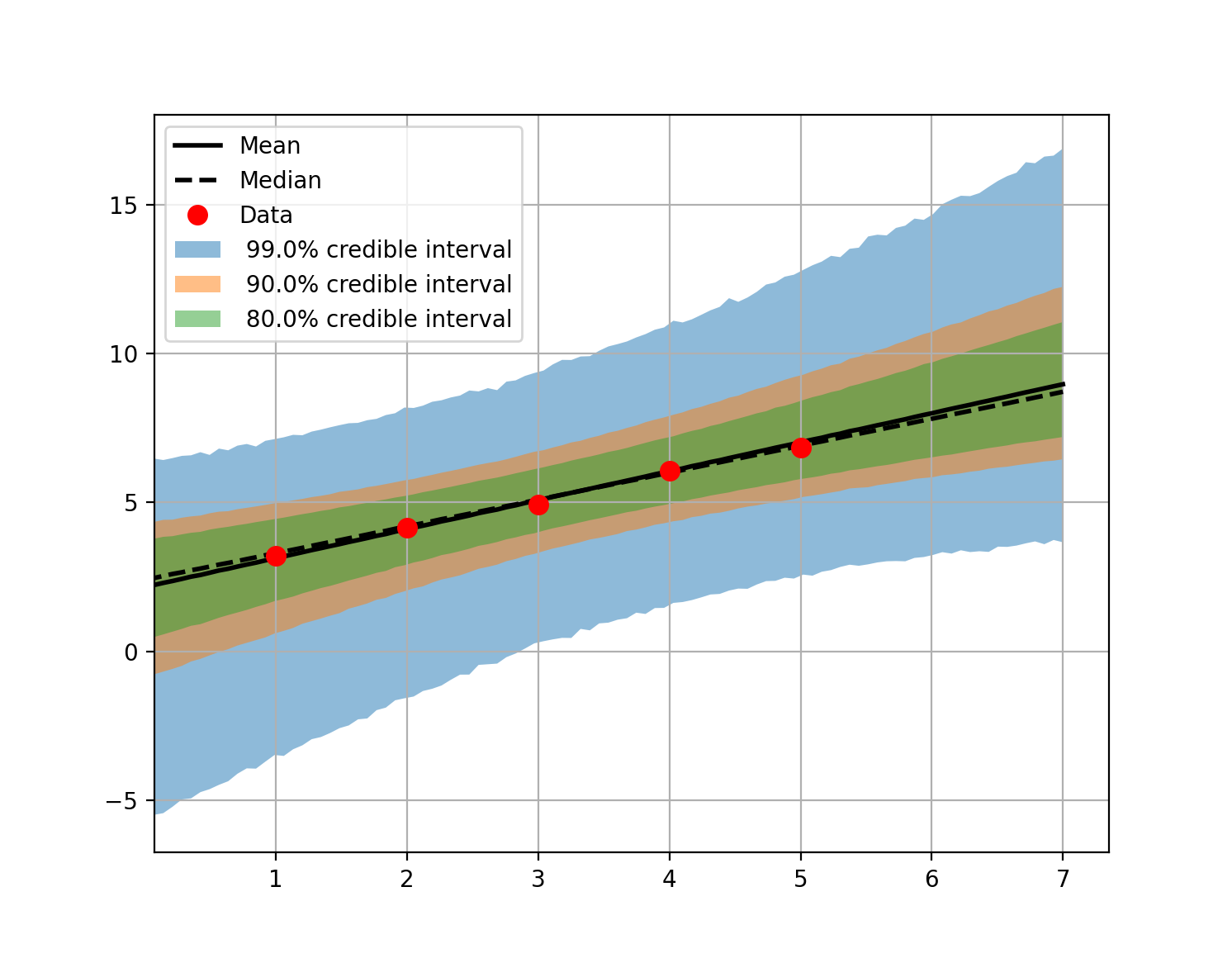
Propagation of Uncertainty
In this tutorial we sample the posterior of a linear problem, as in the Bayesian inference examples. Then we evaluate the linear model for all the parameters that are in the sample database and different input values. We use these model evaluations to compute the uncertainty in the predictions by plotting credible intervals.
The first part is identical to the Bayesian inference example.
For the second part, first we define a new input variable
x = np.linspace(0,7,100)
These are the new points on which we are going to evaluate the linear model on all the samples from the previous step. We define a new function for the propagation that is similar to the one we used for the sampling phase
def model_propagation(s, X):

 a = s['Parameters'][0]
 b = s['Parameters'][1]

 s['sigma'] = s['Parameters'][2]
 s['X'] = X.tolist()
 s['Evaluations'] = []
 for x in X:
   s['Evaluations'] += [a * x + b]
The fields 'sigma', 'X' and 'Evaluations' are going to be saved
for each sample under ['Samples'][k]. In order for these variable
to be saved we have to set
e['Store Sample Information'] = True
Next, we load the json file with the results from the sampling
with open('_korali_result_samples/latest') as f: d = json.load(f)
Then we copy the samples to the Korali variables
e['Variables'][0]['Name'] = 'a'
 e['Variables'][0]['Precomputed Values'] = [ x[0] for x in d['Results']['Sample Database'] ]
 e['Variables'][1]['Name'] = 'b'
 e['Variables'][1]['Precomputed Values'] = [ x[1] for x in d['Results']['Sample Database'] ]
 e['Variables'][2]['Name'] = 'sigma'
 e['Variables'][2]['Precomputed Values'] = [ x[2] for x in d['Results']['Sample Database'] ]
Note that the samples are saved under d['Results']['Sample Database'].
Finally we run the experiment.
Optionally, we can compute the credible intervals and plot the results. You have to uncomment the last two lines of the script.
from plots import *
 plot_credible_intervals('./_korali_result_propagation/latest', data)