Korali Basics
This document describes the basic concepts that make a Korali application.
Creating a Korali Experiment
Korali provides a range of optimization and uncertainty quantification tools. To use these tools, a user needs to create a Korali Experiment. The following python code snippet shows how to load Korali’s library and instantiate a new experiment:
import korali
e = korali.Experiment()
This creates a new experiment object which can be then configured by specifying a Korali problem and solver module combination, as shown below.
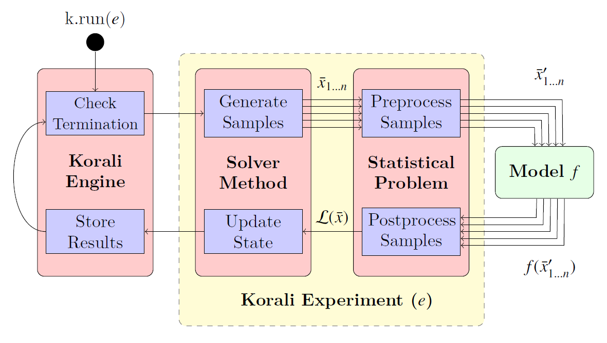
The solver represents a specific algorithm or method find the solution of the specified problem. Most problem types require the evaluation of a computational model (function) to evaluate samples, whose results are returned to the Korali engine.
The cycle of sample creation and evaluation is called a generation. Korali will run as many generations required to reach a certain termination criterion
Experiments contain general settings which affect the way in which Korali runs the experiment and outputs its results.
Korali Problems
A Korali Experiment is configured to run a specific problem type by specifying its problem type setting, for example:
# Example: Setting the experiment to run an optimization problem
e["Problem"]["Type"] = "Optimization"
Sets the experiment to solve an optimization problem. The complete list of problem types can be found here.
Problem Configuration
Each problem type has its own set of properties necessary to be fully described. These settings can be specified by using the following syntax:
# Example: Configuring settings 1 and 2, of string and real types, respectively.
e["Problem"]["Setting 1"] = "String"
e["Problem"]["Setting 2"] = 1.0
Depending on the property, their values could be numeric, text strings, functions, or arrays thereof. They can also contain sub-properties which require their own set of properties, as shown below:
# Example: Configuring setting 3, which contains sub-properties to be defined.
e["Problem"]["Setting 3"]["Sub-Type"] = "myType"
e["Problem"]["Setting 3"]["Parameter 1"] = 0.0
e["Problem"]["Setting 3"]["Parameter 2"] = 1.0
To find the full list of properties for each problem type, look for “Configuration Settings” in the problem’s configuration page. Here is, for example, the configuration settings for Optimization/Stochastic.
Choosing a Solver Method
The next step is to choose which solver algorithm should be used to obtain the results required by the problem. This can be done by specifying the solver type setting.
Solver-Problem Compatibility
Although the complete list of solver types can be found here, each solver can only solve a specific set of problem types. To find which solver methods can be used for a specific problem type, look for “Compatible Solvers” in the problem’s configuration page. Here is, for example, the compatible solvers list for Optimization/Stochastic.
To continue our example above, we will choose to use the DEA, which is a compatible solver for the Optimization/Stochastic problem type.
e["Solver"]["Type"] = "DEA"
It is possible, however, to choose another solver to solve a given problem, simply by changing the solver method choice. For example, if now we wanted to solve the problem using CMAES instead, we simply change the field:
e["Solver"]["Type"] = "Optimizer/CMAES"
Solver Configuration
Korali solvers, just like problems, also contain their own set of settings to configure. For example, CMAES requires defining a population size, the number of samples to run per iteration.:
e["Solver"]["Population Size"] = 32
Termination Criteria
A Korali solver will run until at least one of its termination criteria is met. Termination criteria are entirely user-defined, and can be modified just like any other parameter, for example:
e["Solver"]["Termination Criteria"]["Min Value Difference Threshold"] = 0.0001
e["Solver"]["Termination Criteria"]["Max Generations"] = 1000
Will run iterations of the CMAES algorithm until the difference in objective value (optimization) is less than 0.0001, meaning it has reached convergence within an accepted tolerance OR until it has reached a total of 1000 generations (iterations). The list of termination criteria for each solver can be found in the “Termination Criteria” section of their documentation. Here is, for example, the termination criteria list for CMAES.
Configuration Defaults
Not all the properties or termination criteria of a solver method need to be explicitly defined. Instead, every solver provides a set of defaults values which should work fine in the majority of cases. To see which defaults have been defined for a given method, look for the “Default Configuration” section in their configuration page. Here is, for example, the default configuration for CMAES.
Variables
Most problem types require the description of the parameter-space that represents physical or mathematical phenomenon to analyze. To describe the parameter-space a user needs to define one or more Korali Variable. Variables are created by simply adding their name into the experiment:
# Example: Defining two variables for my problem.
e["Variables"][0]["Name"] = "Thermal Conductivity"
e["Variables"][1]["Name"] = "Heat Source Position"
Variable Configuration
Variable definitions require additional parameters depending on which problem and solver types have been selected. These parameters are explained in detail in each solver/problem documentation page.
For example, the following variable settings are mandatory for the CMAES solver, and these variable settings are mandatory for the optimization problem.
In the code snippet below, we show how the configuration for each variable is specified:
# Example: Defining two variables for my problem and their DEA lower/upper exploration bounds.
e["Variables"][0]["Name"] = "Thermal Conductivity"
e["Variables"][0]["Lower Bound"] = 0.0
e["Variables"][0]["Upper Bound"] = 1.0

e["Variables"][1]["Name"] = "Heat Source Position"
e["Variables"][1]["Lower Bound"] = -10.0
e["Variables"][1]["Upper Bound"] = +10.0
Variable Defaults
Korali problem or solver can specify defaults for their variable settings. To see which variable defaults (if any) have been defined for a given method, look for the “Default Configuration” section in their configuration page. Here is, for example, the variable defaults for CMAES.
Korali Samples and Models
Most problems require defining a model to be optimized/sampled from (among other purposes). A model in Korali is specified as a python function which contains a mathematical formula or an entire computational simulation of a given phenomenon. Model functions accept a single parameter representing a Korali sample. A sample is an input/output object that contains a determinate value for each of the variables defined in the experiment. The syntax to access these values is shown below:
# Defining a model function for my experiment
def myModel(k):
thermalConductivity = k["Parameters"][0]
heatSourcePosition  = k["Parameters"][1]
The sample (k) contains an array of values (Parameters) that hold the value of each variable, in the order as they were defined in the experiment.
Model Output
Different problem types require the output of different results from the model. For example, Optimization/Stochastic requires as output the value of the function at the given point (F(x)), as shown below:
# Defining a model function for my experiment that returns F(x)
def myModel(sample):
thermalConductivity = sample["Parameters"][0]
heatSourcePosition  = sample["Parameters"][1]
distanceFromSource = 1.0 - heatSourcePosition
sample["F(x)"] = thermalConductivity * distanceFromSource * distanceFromSource
Users can also save custom quantities of interest for each samples. These quantities are not used by Korali, but they can be later retrieved from the result files to provide additional data for post-processing.
# Defining a model function for my experiment that returns F(x) and quantities of interest
def myModel(sample):
thermalConductivity = sample["Parameters"][0]
heatSourcePosition  = sample["Parameters"][1]
distanceFromSource = 1.0 - heatSourcePosition
sample["Distance From Source"] = distanceFromSource
sample["F(x)"] = thermalConductivity * distanceFromSource * distanceFromSource
Model functions can also be represented as lambda functions:
# Defining a lambda model function for my experiment that returns F(x)
myModel = lambda sample : sample["F(x)"] = sample["Parameters"][0] * sample["Parameters"][1]
Using the Model
To assign the model to the experiment, the user passes it as parameter to the corresponding setting. For example, for the Optimization/Stochastic problem, we need to define its Objective Function, as follows:
# Setting model to optimize
e["Problem"]["Type"] = "Optimization/Stochastic"
e["Problem"]["Objective Function"] = myModel
Distributions
Some problem type or solvers require the specification of probability distributions. To create distribution, use the following syntax to specify them by name, type, and properties:
# Example: Defining two variables for my problem.
e["Distributions"][0]["Name"] = "My Distribution 1"
e["Distributions"][0]["Type"] = "Univariate/Uniform"
e["Distributions"][0]["Minimum"] = -10.0
e["Distributions"][0]["Maximum"] = +10.0

e["Distributions"][1]["Name"] = "My Distribution 2"
e["Distributions"][1]["Type"] = "Univariate/Normal"
e["Distributions"][1]["Mean"] = 0.0
e["Distributions"][1]["Sigma"] = 5.0
A complete list of distribution types and their configuration can be found here.
Linking Distribution to Variable
Some problems type (e.g., Bayesian) require that variables define a prior distribution. This requires linking a variable to a specific distribution, which can be done by name referencing, for example:
# Example: Linking a variable with its prior distribution
e["Variables"][0]["Name"] = "Thermal Conductivity"
e["Variables"][0]["Prior Distribution"] = "My Distribution 1"
It is possible also to assign the same distribution to different variables:
# Example: Using the same distribution for multiple variables
e["Variables"][0]["Name"] = "Thermal Conductivity"
e["Variables"][0]["Prior Distribution"] = "My Distribution 1"

e["Variables"][1]["Name"] = "Heat Source Position"
e["Variables"][1]["Prior Distribution"] = "My Distribution 1"
Conditional Properties
Some problem types (e.g., Hierarchical Bayesian) require the definition of conditional priors, distributions for which properties are given by the value of a variable, for example:
# Defining conditional prior distributions for a hierarchical Bayesian problem

e["Variables"][0]["Name"] = "Psi 1"
e["Variables"][1]["Name"] = "Psi 2"

e["Distributions"][0]["Name"] = "Conditional 0"
e["Distributions"][0]["Type"] = "Univariate/Normal"
e["Distributions"][0]["Mean"] = "Psi 1"
e["Distributions"][0]["Standard Deviation"] = "Psi 2"

e["Problem"]["Conditional Priors"] = [ "Conditional 0" ]
Running Korali
After the experiment has been fully configured, the user needs to instantiate a Korali Engine object:
k = korali.Engine()
The engine contains all necessary execution logic to run the experiment and produce the results.
Running Experiments
To run a given experiment, simply use the engine’s run() function, passing the experiment as argument.
k.run(e)
It is not necessary to instantiate multiple Korali engines if the application needs to run multiple experiment; it suffices to call the run function as many times as necessary:
k.run(e0)
k.run(e1)
k.run(e2)
Similarly, it is possible to launch multiple experiments simultaneously:
k.run( [e0, e1, e2] )
In this case, Korali will not return until all three experiments have finished.
Running your Korali Application
To run an python application containing a Korali experiment, simply run:
python3 ./myKoraliApp arguments
Accessing Results
When called, the run will not return until one of the experiment’s termination criteria has been met. After return, the experiment will contain a Results section, from which the user can retrieve the desired results.
Each solver type prescribes a different set of results that it produces. To see which results are produced (if any) by a given method, look for the “Results” section in their configuration page. Here is, for example, the results.
To access the results, use the following syntax:
bestSample = e["Results"]["Best Sample"]
print('Found best sample at:')
print('Thermal Conductivity = ' + str(bestSample["Parameters"][0])
print('Heat Source Position = ' + str(bestSample["Parameters"][1])
print('Evaluation: ' + bestSample["F(x)"])
Result Files
After every generation, Korali stores the entire state of the framework (including results) to a results directory. The default path is given in experiment defaults.
To set a different results folder for a given experiment (recommended when you run multiple experiments), use the following syntax:
# Setting a different results folder for my experiment
e["File Output"]["Path"] = "./myResultsFolder"
If you would like to reduce the frequency of state files output or outright disable it, use the follwing syntax:
# Saving results to a file every 5 generations, instead of 1
e0["File Output"]["Enabled"] = True
e0["File Output"]["Frequency"] = 5
e0["File Output"]["Path"] = "/home/user/my.custom.path"

# Disable the output for this other experiment
e1["File Output"]["Enabled"] = False
To preserve the all input/output parameters for every sample generated in Korali, you need to enable it by:
# Saving the details of all samples generated during execution and their results (this file can become really large)
e["Store Sample Information"] = True
This option is by default disabled, since storing all samples may require large file sizes.
Console Verbosity
If you’d like to reduce or increase the amount of information that Korali outputs to console when running, you can use the following syntax:
To set a different results folder for a given experiment (recommended when you run multiple experiments), use the following syntax:
# Do not print anything to console.
e["Console Output"]["Verbosity"] = "Silent"

# Only print important progress notifications to console
e["Console Output"]["Verbosity"] = "Minimal"

# Print all possible information available.
e["Console Output"]["Verbosity"] = "Detailed"
To reduce the output frequency, use the following:
# Print partial results only every 5 generations
e["Console Output"]["Frequency"] = 5
Plotting Results
To generate a plot with the results of your experiment, check the documentation for the Korali Plotter and Korali Reinforcement Learning View tools.